
Hello Friends,
Earlier we explained about Sampling and its distributions and Confidence Intervals. I strongly recommend to go through these articles if you haven’t.
Let us plot some functions and have some fun to understand Normal Distributions. Let’s say we have X-Axis & Y-Axis and we will plot some functions to give an intuition about how to do you look at a particular formula.
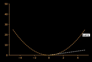
Below Chart represents the Function Y = X i.e. take some value of X and compute the value for Y which is nothing but same value as X. This gives a Linear Line. No matter how complex the function grows, the procedure for plotting is same.

The next function we gonna plot is Y = X². Now how would this plot looks like. Once again we take X = 0 and substitute in the equation and Y turns out to be 0. We continue this steps by substituting different values of X. Say when X = 2, Y becomes 4, similarly when X = -2, Y becomes 4 due to Square in the equation. Hence this function is symmetric in nature (Keep in mind Square always symmetric). Plotting the Values, function looks like below. We can observe gap between X and X² is rapidly increasing. Hence Square equations are little scary!!
Slowly increasing the complexity, lets plot Y = ex. For convenient assume e = 2.7. Substituting different values of X like 0,1,2… Say when X=0, Y=e0 which is equal to 1. Similarly, we can figure out Exponential functions raise very rapidly compared than X & X². This function becomes interesting, when X takes negative value say -1, Y becomes 1/e which approaches to value 0. Therefore when X –> (infinity), Y –> 0. Hence Y = ex is always a positive curve.
 (infinity), Y –> 0. Hence Y = ex is always a positive curve.
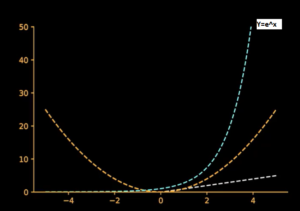
Now, can you imaging what happens when Y = e^(-x). Without thinking based on previous function Y = ex which is positive curve, we can easily guess Y = e^(-x) will be opposite & negative curve. Hence Y = e^(-x) is mirror image of Y = ex.

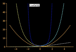
Moving closer to our required function, Y = e^(x^2) i.e. e raise to x square. Based on above charts, we can guess e^(x^2) grows much faster & symmetric than previous functions. I strongly recommend you to substitute different values for X and find Y and try to plot. Notice Y = e^(x^2) at X = 2, we get the value as that of Y = ex when X=4 i.e. twice faster .
.
Finally can we plot Y = e^(-x^2) = [1 /e^(x^2)] i.e. e raise to minus x square. This is a very interesting function. Notice e^(x^2) is in division which means when X becomes high, Y becomes low and vice versa – Inversely Proportional voila ! ! ! In Particular the point at which Y = e^(x^2) had lowest value, that is the point Y = e^(-x^2) have the highest value and vice versa. Below plot shows Y = 20* e^(-x^2).
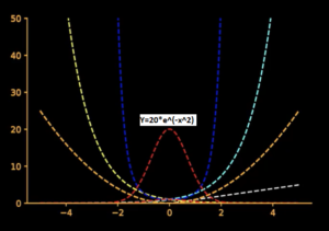
Have you seen this kind of distribution… Ha Ha . Finally we have reached a function which has the shape that we are interested in. This shape we might have seen in many chances in our life – Normal Distribution. Now we know the intuition behind the function Y = e^(-x^2). It tells you that when X increases on either side, this function will fall to 0 and its maximum value will be at X=0.
I hope you enjoyed this article. Leave your comments about your understanding on Normal Distributions. We will come back again with follow up post to deep dive into Normal Distributions. Till then keep studying !!
Wanna More… Try out below books


[…] Diving into Normal Distribution Function Formula Previous Deep Diving into Normal Distribution Function […]
[…] Fun with functions to understand normal distribution […]
[…] Fun with Functions to understand Normal Distribution !! […]
[…] https://ainxt.co.in/fun-with-functions-to-understand-normal-distribution/ […]
You can usually look for a very good deal this avenue.
Think hard and reason out the points for and against your approaches.
A massage session will really relax everybody.
Sure, thanks for feedback.
Every weekend i used to go to see this web page, for the reason that i want enjoyment, since this
this web page conations in fact pleasant funny stuff too.
0mniartist asmr
Good way of telling, and fastidious post to get facts on the topic of my presentation subject matter, which i am going
to deliver in institution of higher education.
asmr 0mniartist
It’s the best time to make some plans for the future and it is time to be happy.
I have read this post and if I could I desire to suggest you some interesting
things or tips. Maybe you can write next articles referring to this article.
I desire to read more things about it! asmr 0mniartist
What’s up, all is going perfectly here and ofcourse every one
is sharing data, that’s actually good, keep up writing.
asmr 0mniartist
Excellent post. I was checking constantly this blog and
I’m impressed! Extremely helpful info specifically the last
part 🙂 I care for such information much. I was looking for this certain info for a very long time.
Thank you and best of luck.
[…] https://ainxt.co.in/fun-with-functions-to-understand-normal-distribution/ […]
[…] https://ainxt.co.in/fun-with-functions-to-understand-normal-distribution/ […]
[…] https://ainxt.co.in/fun-with-functions-to-understand-normal-distribution/ […]
[…] https://ainxt.co.in/fun-with-functions-to-understand-normal-distribution/ […]
[…] https://ainxt.co.in/fun-with-functions-to-understand-normal-distribution/ […]