Hello Friends,
Welcome Back !!
We continue our efforts to provide good articles that makes you to think & help in your professional career as a Data Scientist. Today we are gonna to deep dive into Business Statistics i.e. with the help of Statistics especially “Binomial Distribution” and solve real world challenge and to make statistical decisions.
We expect you to have basic knowledge of Statistics, Random Variables & Distribution functions in order to get most out of this article. You may also read our previous articles to refresh your basics
- https://ainxt.co.in/fun-with-functions-to-understand-normal-distribution/
- https://ainxt.co.in/statistics-and-sampling-distribution-through-python/
- https://ainxt.co.in/measures-of-centrality-facts-and-insights/


Table of Contents
Problem Statement:
Say, you are a Project Manager for ABC Pvt Ltd and forming 3 members team excluding you for a new project. Being the project manager you want to ensure the project meet its objective within agreed SLA otherwise company has to pay penalty of $100,000 to the client depending upon delay in weeks.
In order to achieve to achieve this, you need to ensure there is minimal or no chance of team members attrition. “If one of your team member leaves the project then the project will be delayed by 1 week. If 2 member quits, delay will be 3 weeks. And if all 3 members quits, then the delay will be 6 weeks“.
As typical in any industry, general attrition rate is 20% per year. One of your immediate goal as a project manager is to take a strategy (giving incentives to your team members ) and reduce the attrition rate by 15%. Probability of bringing the attrition by 5% can be at 60%. Can you quantify the risk & calculate possible delay, if any??
Solution
We have 3 members teams(Dinesh, Lakshmi & Partho). These 3 persons can choose to attrite independently i.e. no person choose to stay in the project or attrite based on other persons in the team. We also know the “Probability of Attrite for a person is 20% = 0.2“. Since, these 3 members take decision independently, we have below tree:

- Dinesh has 2 options – Probability of Dinesh Leaves = 20% = 0.2 & Probability of Dinesh Stays in project = 80% = 0.8
- Lakshmi also has 2 options – stay or leave. But Lakshmi’s decision given Dinesh stays or leaves – known as “Conditional Probabilities“. Since each member decision is independent, in our case – they are “Marginal Probabilities“, hence Probability of Leaves=0.2 & Probability of Stays = 0.8.
- Similarly, we have partho decision. Partho decision again can be based on given Dinesh & Lakshmi’s decision. Since independent of each other, again probability remain same i.e. Stays = 0.8 & leaves = 0.2.
Notice the above tree, we have total 8 combinations.
- S1S2S3 i.e. All 3 members stays in the project = 0.8 * 0.8 * 0.8 = 0.512
- S1S2L3 i.e. Dinesh & Lakshmi stays, but partho leaves = 0.8 * 0.8 * 0.2 = 0.128
- S1L2S3 = 0.128
- S1L2L3 = 0.032
- L1S2S3 = 0.128
- L1S2L3 = 0.032
- L1L2S3 = 0.032
- L1L2L3 = 0.008 i.e. all 3 members leave from the project
From above 8 possible combinations, notice we have “Random Variable” – x i.e. No. Of. Persons Leaving from the project.
- x = o Person leaves from the project (S1S2S3) = 0.512
- x = 1 person leaves from the project (S1S2L3 + S1L2S3 + L1S2S3) = 0.384
- x = 2 persons leaves from the project (S1L2L3 + L1S2L3 + L1L2S3) = 0.096
- x = All persons leaves from the project (L1L2L3) = 0.008
Putting these into tables as shown below, we have “Probability Mass function” for the Random Variable we defined.
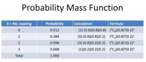
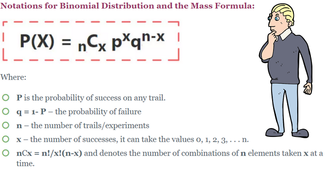
Notice, the probability for each of random variable cases arrived using “Binomial Distribution” Formula
P(x:n,p) = nCx x px (1-p)n-x
where, n: Total no of Trials, x: No of Success i.e. 0, 1, 2, or 3 attritions, p: Prob of Success = 0.2 & (1-p): Prob of Failure = 0.8
Note: For Binomial Distribution, Average: E(x) = np & Variance: V(x) = np(1-p)
Getting into Excel Approach
Using excel is handy to analyze our problem.
First, let us calculate Expected Value of Random Variable x i.e. Mean = E(x) = x * p(x) = [(0*0.512) + (1*0.384) + (2*0.096) + (3*0.008)] = 0.6, using SumProduct formula in excel as shown below:
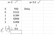
How to interpret E(x) = 0.6 ? If we have large no of projects, each of the projects assume having 3 members in the team, some team there is a chance for 0 people leaving, some teams have chance for 1 people leaving etc… and on average per project the no of people leaving will be 0.6.
Next, from the given problem statement, we know associated delay in the project if team members attrite. Similar to x, delay is also a random variable taking values 0, 1, 3, 6 and it takes probability of 0.512, 0.384, 0.096, 0.008 respectively. Now, Expected value of Delay = E(d) = [(0*0.512)), (1*0.384), (3*0.096), (6*0.008)] = 0.72 using SumProduct formula in excel as shown below:
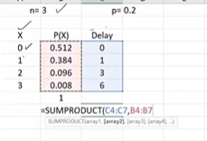
How to interpret E(d) = 0.72 ? This 0.72 represents average delay per project just like average number of people leaving. If we have large no of projects, there will be some project with 0 delay, some have 1 week delay etc… but on average per project will be 0.72 weeks.
Statistical Decisions & Interpretations
Given average penalty per project is $100,000. On average delay per project we found to be 0.72, therefore penalty = 0.72 * $100, 000 = $72,000 will be the penalty on average company is paying to the client.
Remember the project manager’s goal is to reduce the attrition rate from 20% to 15% i.e. probability of success = 0.15, then the probabilities of each random variable x & its mean E(x) & corresponding delay d, E(d) will change as below:
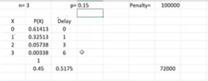
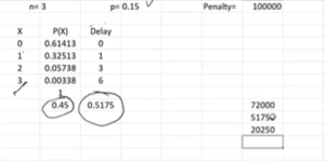
Notice, E(x) = 0.45 i.e. average attrition per project reduced from 0.6 to 0.45 & similarly E(d) = 0.5175 i.e. average delay per project reduced from 0.72 to 0.5175.
Obviously, the penalty paid per project = $100,000 * 0.5175 = $51750. So, money saved from 15% attrition = $72,000 – $51,750 = $20250. So the “cost saved will be the incentive amounts that can be split and shared with team members“.
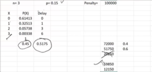
Are we missing something ? Reading the problem statement carefully once again, notice there was a probability associate with the attrition rate coming down from 20% to 15% = 0.6. So, there is still there is a chance for the attrition & delay to remain at older value & penalty will be $72,000.
Therefore $20,250 is not real one. Again we have random variable Expected Penalty = [($72,000*0.4), ($51750*0.6)] = $59,850 using SumProduct formula. Finally the savings will be $72,000 – $58,850 = $12,150.
Now, “you as a project manager can only consider $12,150 as your total savings assuming that the attrition rate will come down from 20% to 15% with 60% chance of happening that can be shared with your team members as incentive“.
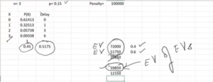
Points to be noted, the value $59,850 is the expected value of Expected values $72,000 & $51,750 i.e. “Average of Averages” !!
Recap
Long journey we have travelled. Let’s quickly summarize the learning’s so far we had
- From given problem, we applied “Binomial Distribution” formula to calculate the Probability of Random Variable x takes value 0,1,2,3 people attritions.
- Making real life inference for taking decisions statistically rather making assumptions.
- Calculating Expected Value of Expected Values – Very important, we gonna come back on this point in our future articles!!


Alright, we hope this article gave a new dimensions to your understanding on statistics and how stats can help us daily in taking decisions. We will continue our journey with this series of “Applied Statistics“. Till we come up with our next one, keep reading !!
- https://ainxt.co.in/measures-of-centrality-facts-and-insights/
- https://ainxt.co.in/measures-of-spreads-range-variance-standard-deviation/
- https://ainxt.co.in/which-college-are-you-likely-to-get-into-a-ml-based-prediction/
- https://ainxt.co.in/hands-on-exploratory-data-analysis-and-prediction/
Credits: This article is originally inspired by Prof. Nagadevera during his Statistics class at ISB.


[…] to do Sampling through Random Sampling Process !! Previous How to do Sampling through Random Sampling Process […]
[…] https://ainxt.co.in/applied-statistics-using-binomial-distribution-for-employee-attrition/ […]