
Hello Friends,
Welcome Back !!
We are excited to deliver quality contents in Data Analytics field through our blog posts. We are talking lot about Statistics especially in our previous posts, which is foundation for becoming Data Scientist. Today we will talk about an important topic, without which no statistical inference is possible – Central Limit Theorem (CLT). You can checkout previous posts on sampling here:
- https://ainxt.co.in/statistics-and-sampling-distribution-through-python/
- https://ainxt.co.in/how-confident-are-you-with-confident-intervals/
- https://ainxt.co.in/fun-with-functions-to-understand-normal-distribution/
- https://ainxt.co.in/applied-statistics-using-binomial-distribution-for-employee-attrition/
- https://ainxt.co.in/how-to-do-sampling-through-random-sampling-process/


Table of Contents
Quick Recap
Especially in previous article, talked “how to do sampling through random sampling process“. Summarizing the key points
- Making inference from Population data is almost impossible, hence we go for Sampling
- Sampling through Random Sampling is best method, however many ways of sampling exists.
- Random Sampling – Each item of Population has same probability of getting included in the sample i.e. Unbiased
- Selection of one sample from population has no influence on selection of other i.e. Independent
- Through Random Sampling, Expected Value of Sampled data E ( x̄ ) will be always equal to mean of the Population data μ i.e. E ( x̄ ) = μ
- And Standard Deviation of Sampled data σx̅ will be equal to Standard Deviation of Population data divided by root of number of samples i.e. σx̅=σ/√n
Introduction
All statistical inferences are made under assumptions that the distribution of given data is Normally Distributed(https://ainxt.co.in/deep-diving-into-normal-distribution-function-formula/). Obviously we deal only with samples and how can we ensure that given sample data will follow Normal Distribution ? Enter – our today’s focus topic “Central Limit Theorem“.
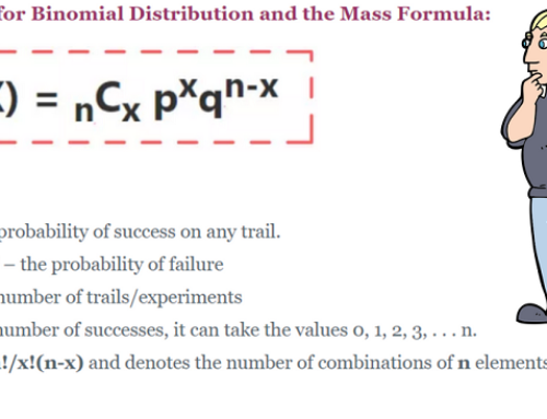
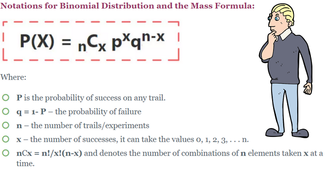
Central Limit Theorem says,
- The Probability Distribution of the Sample Mean
- will be normal when the distribution of data in the population is normal distribution
- will be “approximately normal even if the distribution of data in the population is not normal, under some conditions”
- Mean ( x̄ ) = μ i.e. sampled data mean is same as population mean of raw data
- Standard Deviation ( x̄ ) = σ/√n, where σ is the population standard deviation and n is the sample size
- This is also referred as “Standard Error of the Mean” – represents variation in sample means
- This is also denoted by σx̅ or Sx̅ or SE(x̄)
Testing CLT
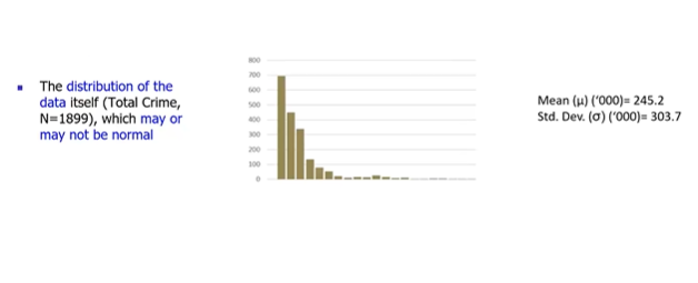
Given a population data of Total Crimes & its impact happened in a City for particular year. Population dataset has total records N = 1899. From below picture, notice that the population data follows Right Skewed Normal distribution with Population Mean 245.2 & Population Standard Deviation 303.7
Do a exercise, pick a sample of 41 records randomly, note down the records, calculate the mean & standard deviation these sample records. Repeat this exercise say, n=10000 times and each time we sample 41 randomly chosen records from total population and record its mean & standard deviation.
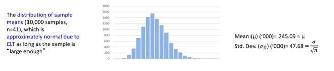
Notice the distribution of Sample means follows Normal Distribution with Sample Mean 245.09 as close with Population Standard Deviation. Standard Error 47.68. Central limit theorem works when the sample is large enough. In our case, we had taken 10,000 samples and each sample has 41 records from total population data.
Note: Standard Error explains variation in the sample means. Lesser the Standard Error, the mean of sample data will be as close as population mean.
“In real world, we wont be given with 10,000 different samples of data to make inference on population. Instead we will do one single random sample with no of sample records, very large enough such that Standard Error is very less. Thereby, we can approximate this single representation of sample data is normally distributed based on Central Limit Theorem and make statistical inference“.
Constraints for CLT
Central Limit Theorem is valid when
- Each data point in the sample is independent of the other
- Sample Size is large enough
- Adequate sample size depends on the distribution of data – primarily its symmetry and presence of outliers
- If the data is quite symmetric and has few outliers, even smaller samples are fine. Otherwise, we need larger samples
Use Case: Application of CLT
Let us solve real world problem using CLT and find interval estimates (Confidence Interval) for a population parameter such as Mean or Population.
Problem Statement:
An online retailer designs silk shirts. They plan for new line of silk shirts ranging between Rs. 2180 and Rs. 8420. The success of this new line depends on the order size in Rs. A sample of 2000 potential customers were randomly selected a campaign is launched. Company received orders from 144 customers. Average Order size is Rs. 6540. Based on previous campaign, assume population standard deviation is Rs. 4608. What can we say about the average order size that will be held after a full fledged market launch?
Solution:
Given – E( x̄ ) = μ = 6540 i.e. sample data average order size; σ = 4608 i.e. Population Standard Deviation
Based on sample data, point estimate for mean of order size is Rs. 6540. But this value might change if we took another sample of 2000 customers. Because of this uncertainty, we go for “Interval Estimate” with associate “Level of Confidence” while predicting Population Parameter.
Interval Estimate: Point Estimate +/- Margin of Error
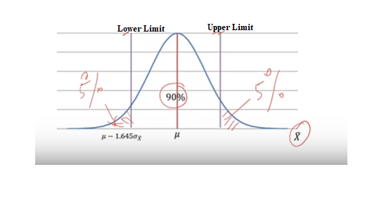
Assume that sample size is large enough so that CLT can be applied. By CLT, distribution of sample mean is x̄ follows normal distribution with μ, σ/√n as shown below. μ we dont know, but we can find Lower Limit & Upper Limit value such that the area under the curve between these 2 limit is 90%.
All we have to do is using standard normal Z-distribution. Since 90% is our area under curve. We left out with 10% error. Since our distribution is Two-Sided, error on each side is 5%. So, the Z Value from table is 1.645. Therefore, Lower Limit = μ-1.645σx̅ and Upper limit μ+1.645σx̅
In other terms, from normal distribution calculations, 90% of all possible sample means will lie within 1.645 standard error of the population mean. Solving,
- P(μ-1.645σx̅ <= x̅ <= μ+1.645σx̅) = 0.90
- P(-1.645σx̅ <= x̅-μ <= +1.645σx̅) = 0.90; Subtracting μ in all terms, Since we wanted to find μ;
- P(-x̅-1.645σx̅ <= -μ <= -x̅+1.645σx̅) = 0.90; Subtracting x̅ in all terms;
- P(x̅+1.645σx̅ >= μ >= x̅-1.645σx̅) = 0.90; Multiply all terms by -1. Note, the direction of distribution changed i.e. < to >;
- P(x̅-1.645σx̅ <= μ <= x̅+1.645σx̅) = 0.90; Flipping back the distribution
We know x̅ = 6540; σx̅ = σ/√n = 4608 /√144 = 344; Now we can substitute these values in above equation to find Lower & Upper Limits.
Turns out, Lower Limit = Rs. 5908 & Upper Limit = Rs. 7172. Therefore, P(5908 <= μ <= 7172) = 0.90; We can say with 90% confidence μ lies in interval between 5908 & 7172.
Based on the sample taken, we got an range where our population average order size will be between these 2 limits with 90% confidence. We can take a strategy whether to go live with new product or not, if this average order size will yield profit to the business.
Note: We can change our confidence level to 95%, 99%. Accordingly find the Z Value and our range will vary. Do try this !!
Conclusion
- To make inference, we do sampling
- Sampling through Random Sampling have E ( x̄ ) = μ & σx̅=σ/√n
- By Central Limit Theorem, even if the population distribution is not normal, the sample data will follow Normal distribution
- Based on this assumption, we make statistical inference on population parameter with some probability or confidence interval attached.
We hope you enjoyed this article. Now it will make sense importance of Sampling, Central Limit Theorem and these important topics helps us to assume and make statistical inference. Will back with another good article soon, till then, Keep Reading !!
- https://ainxt.co.in/introduction-to-collection-principles-and-applications-in-analytics/
- https://ainxt.co.in/importance-of-taylor-series-in-deep-learning-machine-learning-models/
- https://ainxt.co.in/step-by-step-interview-guide-on-decision-tree-algorithm/
- https://ainxt.co.in/deep-learning-on-types-of-activation-functions/
Credits: This article is originally inspired from Prof. Nagadevera during his Statistics class at ISB.


[…] Facts of Cross Entropy Loss in Machine Learning World !! Previous Hidden Facts of Cross Entropy Loss in Machine Learning World […]
[…] https://ainxt.co.in/making-statistical-inference-using-central-limit-theorem/ […]
[…] https://ainxt.co.in/making-statistical-inference-using-central-limit-theorem/ […]