
Hello Friends,
Welcome Back !!
We are writing series of Interview preparations guides on Machine Learning / Artificial Intelligence topics. We have already wrote about regressions. Refer the article links below:
- Linear Regression: https://ainxt.co.in/step-by-step-interview-guide-on-linear-regression-algorithm/
- Logistic Regression: https://ainxt.co.in/step-by-step-interview-guide-on-logistic-regression-algorithm/
Today we will deep dive on one more important Machine Learning Technique – “Decision Tree Algorithm“.


We strongly recommend to refer below articles to have strong basics foundations on Statistics & Machine Learning Framework.
- https://ainxt.co.in/how-confident-are-you-with-confident-intervals/
- https://ainxt.co.in/deep-diving-into-normal-distribution-function-formula/
- https://ainxt.co.in/fundamental-counting-principles-why-we-need-for-analytics/
- Six Modules of any Machine Learning Applications
Table of Contents
What is Decision Tree Algorithm
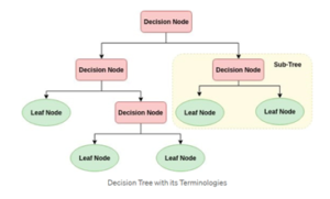
Decision tree is a flowchart-like tree structure where an internal node represents feature, the branch represents a decision rule, and each leaf node represents the outcome. The topmost node in a decision tree is know as the root node. It learns to partition based on the attribute value. It partitions the tree in a recursive manner called recursive partitioning.
Decision Tree Algorithm
- Root Node: It represents the entire population or sample and this further gets divided into two or more homogeneous sets.
- Splitting: It is a process of dividing a node into two or more sub-nodes.
- Decision Node: When a sub-node splits into further sub-nodes, then it is called a decision node.
- Leaf/Terminal Node: Nodes with no children is called Leaf or Terminal node.
- Pruning: When we reduce the size of decision tree by removing nodes, the process is called pruning
- Branch/Sub-Tree: A sub section of the decision tree is called branch or sub-tree.
- Parent and child node: A node, which is divided into sub-nodes is called a parent node of sub-nodes whereas sub-nodes are the child of a parent node.
Advantages
- Easy to understand: Decision tree output is very easy to understand even for people from non-analytical background. Its graphical representation is very intuitive, and users can relate their hypothesis.
- Useful in Data exploration: Decision tree is one of the fastest way to identify most significant variables and relation between two or more variables. With the help of decision trees, we can create new features that has better power to predict target variable.
- Less data cleaning required: Decision tree requires less data cleaning compared to some other modelling techniques. It is not influenced by outliers and missing values to a fair degree.
- Data type is not a constraint: Decision tree is considered to be a non-parametric method i.e., decision trees have no assumptions about the space distribution and the classifier structure.
Disadvantages
- Over fitting: Over fitting is one of the most practical difficulty for decision tree models. This problem gets solved by setting constraints on model parameters and pruning.
- Not fit for continuous variables: While working with continuous numerical variables, decision tree loses information when it categorizes variables in different categories.
Decision Tree – Variants
1) Entropy
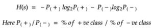
Entropy helps us to build an appropriate decision tree for selecting the best splitter. Entropy can be defined as a measure of the purity of the sub split. Entropy always lies between 0 to 1.
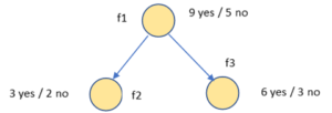
Example: Calculating Entropy for f1 node -3/5 log2 (3/5) – (2/5 log2 (2/5)) = 0.78 bits shown below
2) Information Gain
Information gain is a statistical property that measures how well a given attribute separates the training examples according to their target classification.
The image shown below,
- C is a Pure node
- B is less Impure
- A is more Impure
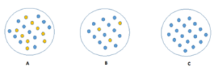
Image A, an attribute with high information gain split the data into groups with an uneven number of positives and negatives and as a result, helps in separating the two from each other.
Information Gain Formula
Here,
Entropy (T) – Entropy value of f1
T – Subset
Tv – Subset after split
Entropy (Tv) – Subset of entropy
Entropy (T) – 8/14 H(f2) – 6/14 H(f3) = 0.91 – 8/14 * 0.81 – 6/14 * 1
Information Gain(f1) = 0.049
3) GINI Impurity
Gini impurity is also somewhat similar to the working of entropy in the Decision Tree. In the Decision Tree algorithm, both are used for building the tree by splitting as per the appropriate features but there is quite a different in the computation of both the methods.

GI = 1 – [(P+)2 + (P–)2] = 1 – [(3/6)2 + (3/6)2] = 1- [0.25 + 0.25]
Therefore, GI = 0.5
Similarly, the same values in Entropy,
 Entropy = -3/9 log 3/6 – 3/6 log 3/6. Therefore, Entropy = 1
Gini index has values inside t
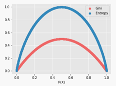
Gini Vs Entropy:
The interval [0, 0.5] whereas the interval of the Entropy is [0, 1]. Computationally, entropy is more complex since it makes use of logarithms and consequently, the calculation of the Gini index will be faster.
Gini Vs Entropy
Decision Tree – Gain Ratio
Information gain is based towards choosing attributes with a large number of values as root nodes. It means it prefers the attribute with a large number of distinct vales. C4.5, an improvement of ID3, user Gain ratio which is a modification of information gain that reduces its bias and is usually the best option. Gain ration overcomes the problem with information gain by taking into account the number of branches that would result before making the split. It corrects information gain by taking the intrinsic information of a split into account.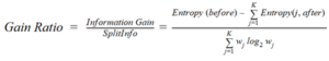
Let us consider if we have a dataset that has users and their movie genre preferences based on variables like gender, group of age, rating et., with the help of information gain, you split at ‘Gender’ (assuming it has the highest information gain) and now the variables ‘Group of Age’ and ‘Rating’ could be equally important and with the help of gain ratio, it will penalize a variable with more distinct values which will help us decide he split at the next level.
How To Avoid Overfitting in Decision Tree
Often you may find that you have overfitted your model to the data, which is often detrimental to the model’s performance when you introduce new data. If there is no limit set of a decision tree, it will give you a zero MSE on training set because in the worse case it will end up making 1 leaf for each observation. Thus, preventing overfitting is of major importance when training a decision tree and it can be achieved in two ways.
- Tree Pruning
- Use a Random Forest
Tree Pruning:
Tree pruning will check for the best split instantaneously and move forward until one of he specified stopping condition is reached.
One of the questions that arise in decision tree algorithm is the optimal size of the final tree. A tree that is too large risks overfitting the training data and poorly generalizing to new samples. A small tree might not capture important structural information about the sample space. However, it is hard to predict when a tree algorithm should stop because it is impossible to tell if the addition of a single extra node will dramatically decrease error.
Pruning should reduce the size of a learning tree without reducing predictive accuracy as measure by a Cross-validation set. There are many techniques for tree pruning that differ in the measurement that is used to optimize performance.
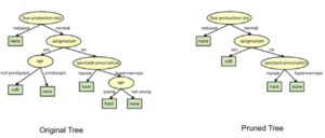
Pruning
Use Random Forest
Random forest is less prone to overfitting and perform better than a single optimized tree.
Bagging is used to create an ensemble of tree where multiple training sets are generated with replacement. In the bagging technique, a data set is divided into N samples using randomized sampling. Then, using a single learning algorithm a model is built on all samples. Later, the resultant predictions are combined using voting in parallel.
Random forest grows multiple trees as opposed to a single tree in CART model. To classify a new object based on attributes, each tree gives a classification and we say the tree ‘votes’ of that class. The forest chooses the classification having the most votes and it case of regression, it takes the average of outputs by different trees.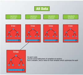
Decision Tee – Performance Matrix
Below are list of Metrics we can be obtained from Decision Tree Algorithm. We have a detailed discussion on below metrics in our Previous article on Logistic Regression. Refer here –>https://ainxt.co.in/step-by-step-interview-guide-on-logistic-regression-algorithm/
- Confusion Matrix
- Accuracy
- Precision
- Recall or Sensitivity
- Specificity
- F1 score
Optimizing the Decision Tree Classifier
- Criterion: optional (default=’gini’) This parameter allows us to use the different-different attribute selection measure. Supported criteria are ‘gini’ for the Gini index and ‘entropy’ for the information gain.
- Splitter: string, optional (default=’best’) This parameter allows us to choose the split strategy. Supported strategies are ‘best’ to choose the best split and ‘random’ to choose the best random split.
- Max_depth: int or None, optional (default = None) The maximum depth or the tree. If None, then nodes are expanded until all the leaves contain less than min_sample_split samples. The higher value of maximum depth causes overfitting, and a lower value cause underfitting.
Thanks for staying there and reading this pocket guide on Decision Tree Algorithm. Hope that we have covered most of the topics related to this algorithm. We hope this helps to refresh your knowledge on this topic. Let us know your feedback on this article and share us your comments for improvements. We will come with interview guide on next topic, till then enjoy reading our other articles.


Very energetic post, I loved that bit. Will there be a part 2?
0mniartist asmr
We are planning 🙂
Truly when someone doesn’t be aware of afterward its up to other people that they will help, so here it happens.
asmr 0mniartist
My brother recommended I may like this website. He was once entirely right.
This put up truly made my day. You cann’t consider simply how so much time I had
spent for this info! Thank you! 0mniartist asmr
Thanks, keep reading our article
If you are going for finest contents like me, simply pay a visit this web site daily
because it offers feature contents, thanks 0mniartist asmr
hi!,I love your writing very so much! percentage we keep up a correspondence extra about your post on AOL?
I require a specialist in this area to unravel my problem.
Maybe that is you! Having a look forward to see you.
asmr 0mniartist
Sure !!
Wonderful web site. Plenty of useful info here.
I’m sending it to several friends ans additionally sharing in delicious.
And obviously, thanks to your sweat! asmr 0mniartist
Hi I am so happy I found your blog page, I really found you by accident, while
I was browsing on Digg for something else, Anyways I am here now and would
just like to say many thanks for a marvelous post and
a all round enjoyable blog (I also love the
theme/design), I don’t have time to read it all at the
moment but I have bookmarked it and also included your RSS feeds, so when I have time I will be back to read a lot
more, Please do keep up the awesome work. asmr 0mniartist
Hmm it seems like your site ate my first comment
(it was extremely long) so I guess I’ll just sum it up what
I had written and say, I’m thoroughly enjoying your blog.
I too am an aspiring blog writer but I’m still new to
everything. Do you have any helpful hints for newbie blog writers?
I’d certainly appreciate it.
[…] https://ainxt.co.in/step-by-step-interview-guide-on-decision-tree-algorithm/ […]