Step by Step Interview Guide on Logistic Regression Algorithm !!

Hello Friends,

Welcome Back !!

In series of our Interview preparations guides on Machine Learning / Artificial Intelligence topics, last article we saw about Linear Regression.

• Refer the article here –> https://ainxt.co.in/step-by-step-interview-guide-on-linear-regression-algorithm/

Today we will deep dive on important topics related to “Logistic Regression”  in interview perspective. We also published a detailed python notebook that explains applying Logistic Regression to a dataset and predict whether a student gets admission or not.

• Refer the article here –> https://ainxt.co.in/which-college-are-you-likely-to-get-into-a-ml-based-prediction/

We strongly recommend to refer below articles to have strong basics foundations on Statistics & Machine Learning Framework.

• https://ainxt.co.in/how-confident-are-you-with-confident-intervals/
• https://ainxt.co.in/deep-diving-into-normal-distribution-function-formula/
• https://ainxt.co.in/fundamental-counting-principles-why-we-need-for-analytics/
• Six Modules of any Machine Learning Applications

Definition: Logistic Regression

Logistic regression is a statistical model uses a logistic function to model a binary dependent variable. Mathematically, a binary logistic model has a dependent variable with two possible values, such as pass/fail which is represented by an indicator variable, where the two values are labeled “0” and “1”.

• It predicts the probability of an event occurring
• Approach is very similar to regression
• Predicted probabilities are always between 0 and 1

Advantage of Logistic Regression

1. Good accuracy for many simple data sets and it performs well when the dataset is linearly separable.
2. It makes no assumptions about distributions of classes in feature space.
3. Logistic regression is less inclined to over-fitting, but it can overfit in high dimensional datasets. One may consider Regularization (L1 and L2) techniques to avoid over-fitting in these scenarios.
4. Logistic regression is easier to implement, interpret, and very efficient to train.

Disadvantage of Logistic Regression

1. Sometimes Lot of Feature Engineering Is required
2. If the independent features are correlated it may affect performance
3. It is often quite prone to noise and overfitting
4. If the number of observations is lesser than the number of features, Logistic Regression should not be used, otherwise, it may lead to overfitting.
5. Non-linear problems can’t be solved with logistic regression because it has a linear decision surface. Linearly separable data is rarely found in real-world scenarios.
6. It is tough to obtain complex relationships using logistic regression. More powerful and compact algorithms such as Neural Networks can easily outperform this algorithm.
7. In Linear Regression independent and dependent variables are related linearly. But Logistic Regression needs that independent variables are linearly related to the log odds (log(p/(1-p)).

Assumptions

1. Appropriate outcome structure

Binary logistic regression requires the dependent variable to be binary and ordinal logistic regression requires the dependent variable to be ordinal.

2. Observation independence

Logistic regression requires the observations to be independent of each other

3. Linearity of independent variables and log odds

Linear relation between independent variable and the Log odds

4. Large Sample size

Logistic regression typically requires a large sample size

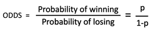
Interpret Odds ratios in Logistics Regression

Odds and Probability

Odds are the ratio of something happening to something not happening.  Whereas, Probability is the ratio of something happening to everything that could happen.

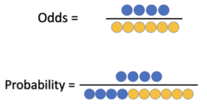
Odds Probability

Odds of winning = 4 / 6 = 0.6666

Probability of winning = 4 / 10 = 0.40

Probability of losing = 6 / 10 = 0.60 (1 – 0.40) = 0.60

Given the Probability, we can also calculate the Odds as below,

Odds Probability Formula

Now, we increase the total number of games played from 10 to 100 and I am still able to win only 4 out of these 100 games,

            Odds of winning = 4 / 96 = 0.0417

If we further increase the number of games to 500, and my number of wins stay the same, the odds now become,

            Odds of winning = 4 / 496 = 0.0081

On the other hand, if I start beating the games and loses the same 6 of those while I win the rest,

            Odds of winning = 94 / 6 = 15.667

And similarly, for 500 games,

            Odds of winning = 494 / 6 = 82.3333

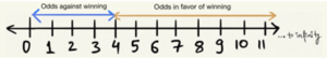
Odds Comparison

Log Odds

Log Odds is nothing but log of odds, i.e., log(odds).

Odds of winning = 4 / 6 = 0.6666

Log(Odds of winning) = log(0.6666) = -0.176

Odds of losing = 6 / 4 = 1.5

Log(Odds of losing) = log(1.5) = 0.176

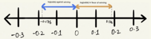
Logs Odd

The log function helped us making the distance from origin(0) same for both odds.

Logit Function

The logit function is simply the logarithm of the odds. The value of the logit function heads towards infinity as ‘p’ approaches 1 and towards negative infinity as it approaches 0.  The logit function is useful in analytics because it maps probabilities (which are values in the range [0, 1]) to the full range of real numbers. In particular, if you are working with ‘yes or no’ inputs it can be useful to transform them into real-valued quantities prior to modelling.

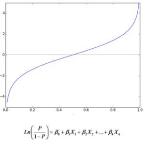
Logit Function

Sigmoid Function

The inverse of the logit function is the Sigmoid function, if you have a probability p, sigmoid(logit(p)) = p.  The sigmoid function maps arbitrary real values back to the range [0, 1]. The sigmoid might be useful if you want to transform a real valued variable into something that represents a probability.

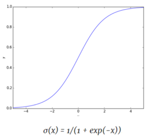
Sigmoid Function

Logistic Regression Performance Matrix

1) Confusion Matrix

Confusion matrix is a table that is often used to describe the performance of a classification model on a set of test data for which he true values are known.

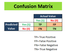
Confusion Matrix

True Positive (TP): Actual label for that column was ‘Yes’ in the test dataset and our logistic regression model also predicted ‘Yes’.

True Negative (TN): Actual label for that column was ‘No’ in the test dataset and our logistic regression model also predicted ‘No’

False Positive (FP): Actual label for that column was ‘No’ in the test dataset but our logistic regression model predicted ‘Yes’

False Negative (FN): Actual label for that column was ‘Yes’ in the test dataset but our logistic regression model predicted ‘No’

confusion Matrix formula

2) Type 1 Error

Type 1 error is also known as a False Positive (FP) and occurs when a classification model incorrectly predicts a true outcome for an originally false observation.

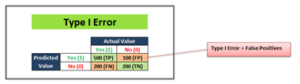
Type I Error

3) Type II Error

Type II error is also known as a False Negative and occurs when a classification model incorrectly predicts a false outcome for an originally true observation.

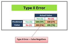
Type II Error

4) Accuracy

Accuracy is the proximity of measurement results to the true value. It will describe how accurate our classification model is able to predict the class labels given in the problem statement. Accuracy = (TP + TN) / Total Customers

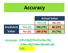
Accuracy

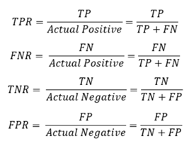
5) Recall or Sensitivity

Out of the total positive, what percentage are predicted positive.

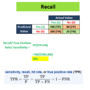
Recall Formula

6) Precision

Out of all the positive predicted, what percentage is truly positive.

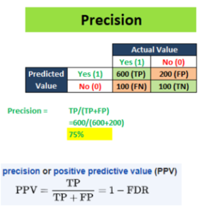
Precision formula

7) Specificity

Specificity measures the proportion of actual negatives that are correctly identified as such.

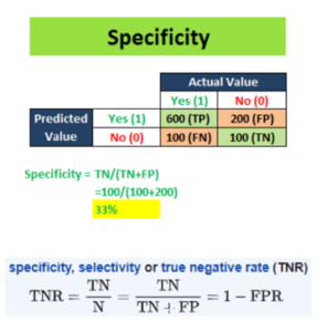
Specificity Formula

8) F1 Score

F1 score is a measure of a test’s accuracy. It considers both the precision p and the recall r of the test to computer the score

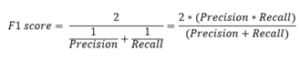
F1 Score formula

9) ROC Curve – AUC Score

Area under the Curve – AUC; Receiver Operating Characteristics Curve – ROC. ROC Curve can be visualizing a classification model by assigning its different thresholds to create different data points to generate the ROC Curve.  The area under the ROC curve is known as AUC. The more AUC the better your model is.  The ROC-AUC can help us judge the performance of our classification models as well as provide us a means to select one model from many classification models.

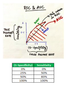
ROC and AUC

Logistic Regression Optimization

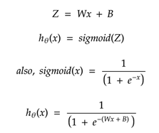
Logistic Regression uses probabilities to classify the data, its similar to linear regression expects it uses sigmoid function instead of the linear function.

Hypothesis function = hӨ(x) = sigmoid(Z)

Since the output of sigmoid function lies in the range [0, 1], hence the logistic regression always results in values lying in the range [0, 1].

Logistic Regression Optimization

Cost Function for Logistic Regression

Cost function describes how good is our model at making predictions for the given dataset. We try to minimize cost function in order to develop an accurate model with minimum error. In linear regression, we use mean square error, which results in the convex cost function, but if we use mean square error in logistic regression, the cost function will end up being non-convex, with many local minima, and in such cases, gradient descent fail to optimize cost function properly as it may end up choosing any local minima as global minima instead of the actual global minima.

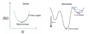
Convex vs Non Convex

Hence in the case of logistic regression, we cannot use the mean square error function.

Linear regression uses the below cost function,

We can redefine J(Ө) as

Appropriately, is the sum of all the individual cost over the training data. To further simplify,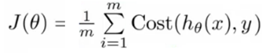

If we use this function for logistic regression this is a non-convex function for parameter optimization. Our hypothesis function has a non-linearity (sigmoid function of hӨ(X))

A convex logistic regression cost function,

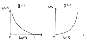
After, combining them into one function, the new cost function is,

We know that there are only two possible cases,

In summary, our cost function for the Ө parameters can be defined as,

We simplify the above notation, using gradient descent,

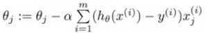
Logistic Regression Cost Function

Thanks for staying there and reading this pocket guide on Logistic Regression. Hope that we have covered most of the topics related to Logistic Regression. We hope this helps to refresh your knowledge on this topic. Let us know your feedback on this article and share us your comments for improvements. We will come with interview guide on next topic, till then enjoy reading our other articles.