Hello Friends,
Welcome Back !! I took some time to choose an interesting topic for our readers to benefit. We have been talking around in general topic related to analytics and this time i wanted to focus on one of the fundamental mathematic concepts we read during our school days, yet we not sure where it has been applied in real world applications – "Taylor Series".
Earlier in my previous article – https://ainxt.co.in/six-modules-of-any-machine-learning-applications/, we talked about 6 jars of any Machine Learning Models – Data, Tasks, Models, Loss Functions, Learning Algorithm & Evaluation. Today we will uncover, how "Taylor Series" applied in Loss Functions for effective learning models particularly in the context of Deep Learning Models.
To get into the basics, Refer our previous articles highlighted below, in order to make most out of this article.
- https://ainxt.co.in/six-modules-of-any-machine-learning-applications/
- https://ainxt.co.in/deep-learning-on-types-of-activation-functions/
- https://ainxt.co.in/temperature-prediction-with-tensorflow-dataset-using-cnn-lstm/


Table of Contents
Introduction
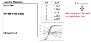
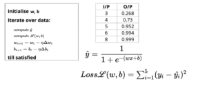
In a nutshell, Learning Algorithms are how effectively our Machine Learning models able to understand the mapping between Input Variables vs Output Predictor variables. Consider below example, in order to predict O/P from given I/P values, we used Sigmoid Function 1 / 1 + e ^-( (w*x ) + b) (To know more about this – Refer our earlier article –> https://ainxt.co.in/deep-learning-on-types-of-activation-functions/ ) as our learning function.
Now learning algorithm will iterate with different values "w" (the slope) & "b" (the intercept) and compute the loss function i.e. difference between predicted output values vs original output values for a given inputs.
Random Guessing
What is the best way to determine w & b such that loss function achieved global minimum value ?
Earlier we started with "Random Guess" of w & b values (say begin with 0). Lets say this loss value is our baseline value. Next we will slightly increase/decrease the value of w & b such that w = w+/- Δw & b = b +/- Δb. This new w & b might reduce the loss or can increase the loss, depending on which our next guess depends on.
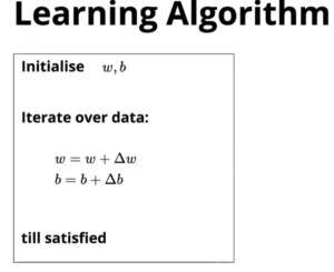
The only problem in this manual guess approach is Δw & Δb is coming from random guess and we cant assure of guess will reach us to global minimum after certain iterations. Also we cant afford to run operations for more number of times.
Hence, we need a more principle way of "calculating loss which is guided by mathematical loss functions". Our objective is whenever we change the value of w & b, we want to ensure that loss is steadily decreasing.
Mathematical Approach
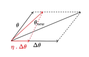
So, Let's assume a vector θ = [w, b] and want to find optimal vector Δθ = [Δw, Δb] by changing different values of w & b. While changing the values of w & b, we want to ensure the change in values is very small. Hence we multiply η with Δw, Δb where η –> Step Controller such that θ = θ +/- η*Δθ.
Now the question still remain how do i get the Δθ in a principled manner, so that every point when i compute loss L(θ)new with new values of w & b should be less than L(θ)old i.e. L(w) > L(w+η*Δw). We need to prove that new Δw, Δb values loss values less than previous values. This opens up our interest of today's topic "Taylor Series".
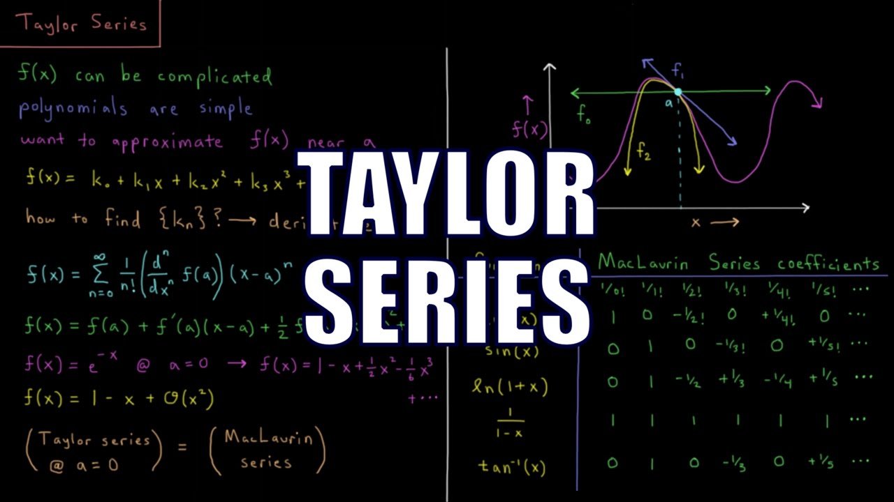
Taylor Series Introduction
What Taylor Series tells us that if you have a function f(x) and if you know that value of that function at certain point(say x), then it's value at new point which is very close to x, can be given by below expression

Now lets correlate this equation with our problem. We are going to take a small step away from w i.e. Δw and we want to make sure the loss decreases. Voila!!!!!!! Taylor series actually helps to find the next small step. How ? Let's breakdown !!
If you notice the formula of Taylor Series, the function value after the small step f(x+Δx) as compared to function before small step f(x) is "f(x) + Sum Of Other Values" as highlighted below. This "Sum of other values" actually depends on Δx. If Δx is such that "Sum of Other Values" that is adding to f(x) to be negative, then the new loss f(x+Δx) < f(x).
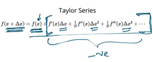
So, we need to find Δx such that right side of equation -ve. The more -ve, the more better. f'(x), f"(x), f"'(x) –> are derivatives of given input function f(x).
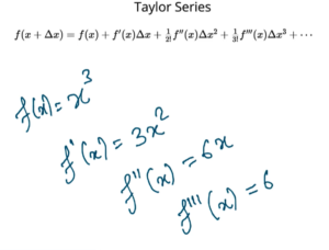
Example: Let f(x) = x^3 then 1st Order derivative f'(x) = d/dx(f(x))=3*x^2, similarly 2nd Order derivative f"(x) = d/dx(f'(x))=6x
Note: Now you can assume value for x (say x=3) and very small step size Δx (say Δx=0.0001) and substitute in Taylor series formula and see if loss value decreased or not. If not, then our assumption of Δx is not good.
More Intuitions about Taylor Series
To make more sense, i replaced function f with L that denotes loss function & replaced x & Δx with w & Δw –> slope loss value we try to minimize.
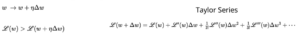
Again i repeat, crux of taylor series is somehow we need to find Δw, so that "Sum of Other Values" turns to be -Ve. Then new loss will be small than previous value.
In above formula, we represent only scalar loss function i.e. only for slope w, but we know we have to compute new value for intercept b also, hence we represent the Taylor Series as Vector θ = [w, b]
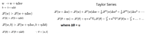
Note: We replaced Δθ –> u, L(θ+Δu) –> Loss at new value of θ, which is equal to Old value L(θ) + [Sum of Other Values].
Let's simply our new Vector – Taylor Series Formula, we know η will always be very small (say η = 0.0001). If so next higher order terms like η^2, η^3 will be very very small, hence can be approximated to 0.
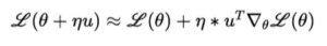
Now all our job is to find the value of u i.e. Δθ , such that η*u^T*Δθ*L(θ) will be negative.
Partial Derivatives To Gradient’s
By comparing Δθ*L(θ) analogy with Original Taylor Series Equation, it is 1st order partial derivative since θ is a vector of [w, b] i.e. vector with 2 variables.
What is Partial Derivatives ? Lets start with derivative function f(w) = w^3, then 1st order derivative d/dw(f(w))= 3*w^2. But i now have a function dependent on 2 variables f(w, b) = w^3 + b^2. In this case, we can find derivative with respect to w first and with respect to b separately, called as Partial Derivatives.
Hence,
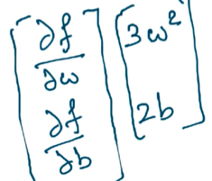
Going back, Δθ*L(θ) is nothing but collection of partial derivatives with respect to w & b. We know L(θ+Δu) –> Real No , L(θ) –> also a real no , η –> also a real no , hence u^T*Δθ*L(θ) should also be a real no !!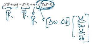
Gradient Descent Update Rule
So far we have came to, L(θ+η*u) = L(θ) + η*u^T*Δθ*L(θ). We are yet to find the value of u such that η*u^T*Δθ*L(θ) becomes -Ve.
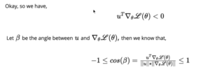
Rewriting above equation as L(θ+η*u) – L(θ) = η*w. The New move η*u would be favorable only if, L(θ+η*u) – L(θ) < 0 implies u^T*Δθ*L(θ) < 0. 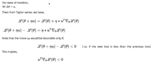
u is vector of [w, b] and Δθ*L(θ) is again a gradient vector of partial derivatives with respect to w & b as saw earlier. Whenever a dot product happens between 2 vectors, there involves "Cos Angle – β" between these 2 vectors given as below:
We are interested only in Numerator, hence multiply throughout by denominator, we get
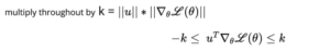
we want u^T*Δθ*L(θ) as negative as possible and maximum negative we can achieve -k and this will happen only when cos angle -β between 2 vectors is -1. From elementary mathematics, Cos = -1 then β = 180 degrees. 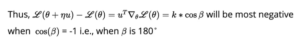
Thus, Gradient Descent Rule,
- The direction u that we intend to move in should be 180 degree with respect to the gradient
- In other words, move in a opposite direction to the gradient
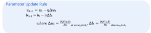
Updated Parameter Rule
Now our parameter update rule looks like find the gradients Δw & Δb and move in opposite direction, hence "-" in the formula.
Complete Learning Algorithm
Finally, we saw the update rule where the vector u and gradient vector should be opposite to each other i.e. u = -Δθ*L(θ) so that angle between them is 180 degrees. So we have data i/p & original o/p given, fitted in a model that uses sigmoid function. Now we use the update rule such that Loss function reaches global minima.
We initialize random w, b values first and substitute in sigmoid function and find the predicted o/p & compute Loss function L(w, b) i.e. sum of squares of difference between Original Vs Predicted Output values. Once we have the loss function, we can find the derivative of Loss function with respect to w & b i.e. Δw =
We can fix step size η such that Δw & Δb are very very small. Using this we can find new w & b which when plugged in sigmoid function, the loss between previous predicted outcome vs new predicted outcome is actually lesser. We will iterate over certain steps such than there is no improvement in loss values, we reached our minima.
Conclusion:
Almost every machine learning algorithm one or other way uses Gradient Descent Optimization to compute loss function such that our models performs better. Taylor Series is actually behind Gradient Descent Rule Algorithm. We might have studied Taylor Series in our school days but without understanding the intuitions / logic behind and its practical application. We also noticed that we used little bit of trigonometry like cos , dot products which in turn helps to come to our derive the final rules.
I hope this article gives you a new source of information and do let us know your kind feedback to improvise further. I have taken inspiration from IIT professor Mithesh Khapra's original course on Deep Learning offered at https://padhai.onefourthlabs.in/ for this article.
Do check his course for more information. We will back with next article, till then keep reading our other articles 🙂
- https://ainxt.co.in/deep-learning-on-types-of-activation-functions/
- https://ainxt.co.in/vectors-and-matrices-why-do-we-care-for-them-in-analytics/
- https://ainxt.co.in/understanding-feature-selection-for-model-accuracy-in-regression/
- https://ainxt.co.in/complete-guide-to-clustering-techniques/


[…] https://ainxt.co.in/importance-of-taylor-series-in-deep-learning-machine-learning-models/ […]
[…] https://ainxt.co.in/importance-of-taylor-series-in-deep-learning-machine-learning-models/ […]
[…] https://ainxt.co.in/importance-of-taylor-series-in-deep-learning-machine-learning-models/ […]
[…] https://ainxt.co.in/importance-of-taylor-series-in-deep-learning-machine-learning-models/ […]
[…] https://ainxt.co.in/importance-of-taylor-series-in-deep-learning-machine-learning-models/ […]