Hello Friends,
Welcome to this tutorial on Deep Diving into Normal Distributions. This blog post is continuation of our previous blog post “Fun with functions to understand Normal Distribution“. I strongly recommend you to have a look on this post first before continuing further as you might first need to understand the mathematical functions behind Normal Distribution.
Alright !! Lets begin.
Remember the plot below ? The function Y = e^(-x^2) = [1 /e^(x^2)] i.e. e raise to minus x square has the shape that we are interested in – Normally Distributed. Recall When X = 0, Y = 1 i.e. Maximum value. As we keep increasing the value of X, value of Y will drop and also symmetric. Why it is Symmetric – because of “Square” in the equation. Why Y decreasing – because of “Minus” in the equation.

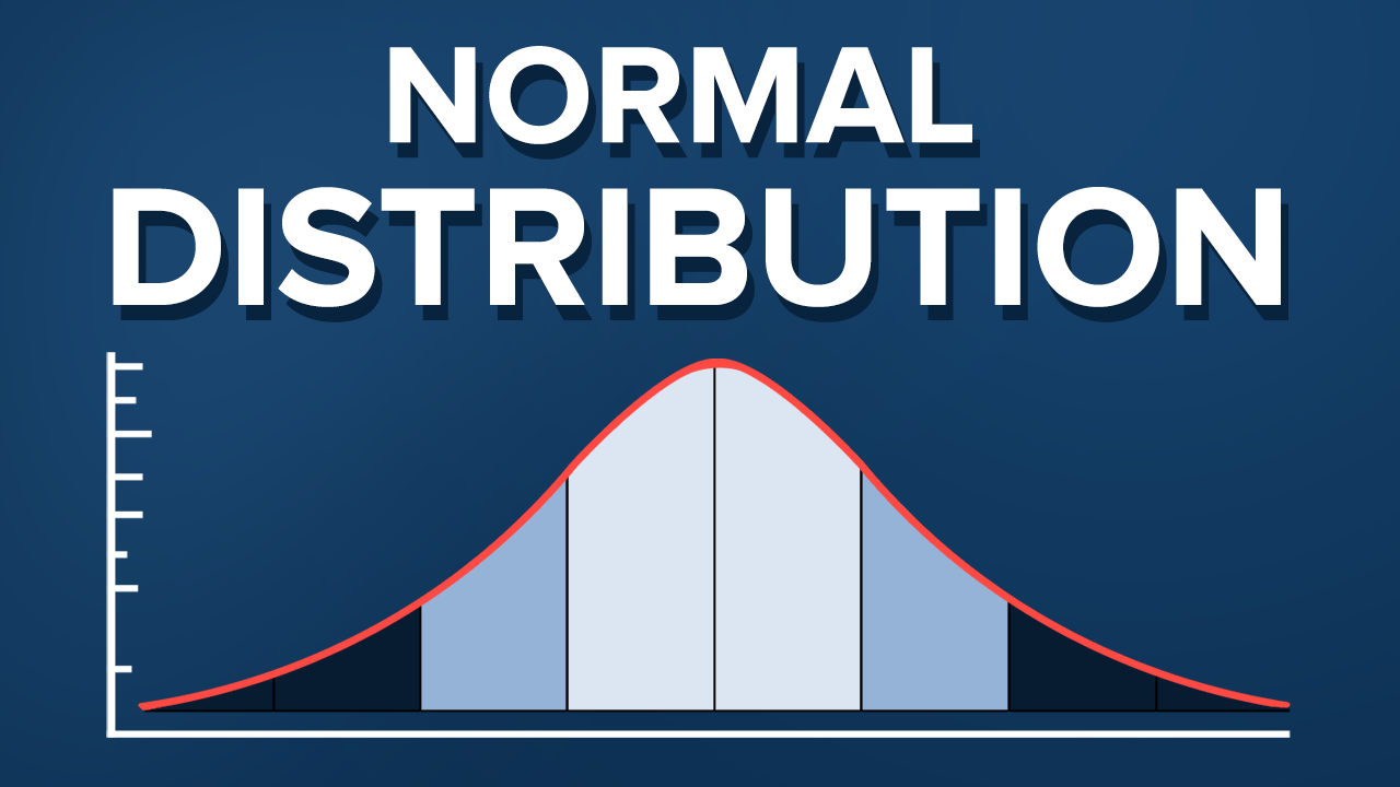
This kind of Shape where Peak in the Middle and dropping on either sides symmetrically is commonly found in many scenarios. Example – Scoring runs in cricket. We can see a rare chance of individual cricketer scores less than 10 runs & also scoring century. Often we can find average score has peak in middle in the range of 40-60 runs.
Having said that, I will introduce you now the formula for Normal Distributions – Probability Density Function (PDF).

Probability Density Function Formula for Normal Distribution
Note: Q1) In above PDF equation shown, new term “1/2π” was introduced? Where does it comes from ?
Q2) Also, notice the term ![]() . What does that 0, 1 represent ?
. What does that 0, 1 represent ?
To find the answer, lets explore the properties of PDF.
Any Probability Density Function pdf f(x) should satisfy 2 properties:

PDF properties
Property1: Function f(x) value should always greater than 0. We already saw in previous article that e^(-x^2) is always positive irrespective of value of X.
Property2: If we Integrate e^(-x^2) over -infinity to +infinity, we get 2π. Watch this Video for proof. To satisfy the property, value should be 1. Hence we bought additional 1/2π in the PDF equation. This answers our first question – Q1.
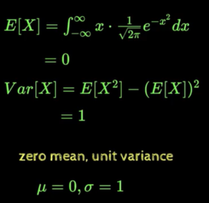
To Answer our Second Question – Q2, lets calculate Expected Value & Variance of the density function.

It turns out that Expected Value of PDF of Normal Distribution is “0” (recall symmetric nature, positive & negative will cancel out i.e. center of gravity is around zero). Similarly Variance is “1”. Now ![]() is referred as “Normal with Zero Mean and Unit Variance” density function.
is referred as “Normal with Zero Mean and Unit Variance” density function.
Table of Contents
Normal Distribution(Changing μ):
Here, we will vary different values of Mean keeping unit Variance constant. Formula looks as below. How did we arrive this ?

Lets substitute different values for μ. Notice the distribution gets shifted based on μ value.

Normal Distribution(Changing σ2):
Here, we keep zero mean, but try to vary different values of variance. Formula looks as below:

Lets substitute different values for σ. Notice the distribution gets different peakness based on σ value.

To summarize, changing μ will shift the distribution & changing σ will shrink or grow more.
Finally,
General Normal Distribution(Changing μ & σ2):
It’s the combination of above 2 formula’s. Using this we can vary different values of μ and σ and get different combinations of Normal Distributions.

Hope, you have gained how Normal distribution is evolved using Mathematics. Kindly leave your comments. We strongly recommend to go through below books to gain further knowledge.


Very good explanation
Thanks
you forgot the sigma in front Sqrt 2xpi
Thanks for Valuable comments. However i am not able to get where exactly you are referring. Could you explain more on your point, so i can address it.
In the last formula of normal distribution,: “General Normal Distribution(Changing μ & σ2):…”
[…] Deep Diving into Normal Distribution Function Formula […]
[…] Deep diving into normal distribution function formula […]
[…] https://ainxt.co.in/deep-diving-into-normal-distribution-function-formula/ […]
Hello would you mind stating which blog platform you’re using?
I’m looking to start my own blog in the near future but I’m having a hard time choosing between BlogEngine/Wordpress/B2evolution and Drupal.
The reason I ask is because your layout seems
different then most blogs and I’m looking for something unique.
P.S My apologies for getting off-topic but I had to ask!
0mniartist asmr
We are using WordPress and installed Avada Theme for this website.
Hi there to every one, as I am truly keen of reading this website’s post to be updated regularly.
It contains good data. 0mniartist asmr
I think this is among the most important info for me.
And i am glad reading your article. But should remark on some general things, The site style is wonderful, the
articles is really great : D. Good job, cheers 0mniartist asmr
Glad u liked our articles, keep reading !!
Great work! That is the type of information that are supposed to be shared around the web.
Disgrace on Google for no longer positioning this publish
higher! Come on over and talk over with my website . Thank you =) asmr 0mniartist
I have been reading out many of your stories and i can state clever stuff. I will definitely bookmark your site.
I¡¦ve recently started a blog, the info you provide on this site has helped me tremendously. Thanks for all of your time
Normally I do not learn post on blogs, however I wish to say that this write-up very forced me to take a look at and do so! Your writing style has been amazed me. Thanks, quite great article.
Thank you for sharing excellent informations. Your web-site is so cool. I’m impressed by the details that you have on this blog. It reveals how nicely you perceive this subject. Bookmarked this website page, will come back for more articles. You, my pal, ROCK! I found simply the information I already searched everywhere and simply could not come across. What a great site.
Its like you read my mind! You appear to know a lot about this, like you wrote the book in it or something. I think that you can do with some pics to drive the message home a bit, but instead of that, this is wonderful blog. A great read. I’ll definitely be back.
I am not sure where you are getting your info, but great topic. I needs to spend some time learning more or understanding more. Thanks for excellent information I was looking for this information for my mission.
[…] https://ainxt.co.in/deep-diving-into-normal-distribution-function-formula/ […]
[…] statistical inferences are made under assumptions that the distribution of given data is Normally Distributed(https://ainxt.co.in/deep-diving-into-normal-distribution-function-formula/). Obviously we deal only […]
[…] https://ainxt.co.in/deep-diving-into-normal-distribution-function-formula/ […]
[…] https://ainxt.co.in/deep-diving-into-normal-distribution-function-formula/ […]