Hello Friends,
Welcome Back !!
Once again i am excited to come up with another interesting topic in Deep Learning or Machine Learning world – “Information Theory – Cross Entropy” which many of us not aware of its applications & uses.
To understand about Cross Entropy loss, we need our basic foundations which we have discussed a lot through our articles like importance of Probability, Statistics, Expected Value etc… in Analytics. Snatch our previous articles here –>
- https://ainxt.co.in/making-statistical-inference-using-central-limit-theorem/
- https://ainxt.co.in/importance-of-taylor-series-in-deep-learning-machine-learning-models/
- https://ainxt.co.in/statistics-and-sampling-distribution-through-python/
- https://ainxt.co.in/fundamental-counting-principles-why-we-need-for-analytics/
Table of Contents
Random Variable – Recap
“Random Variable” is a function which maps each outcome in an event Ω to a value associated with it.
Example: As shown below, a random variable G which maps each student to one of the possible 3 values with probability associated with it.
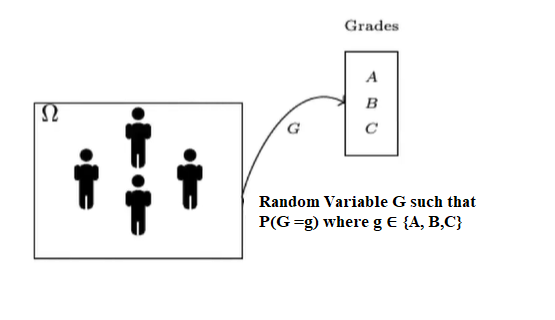
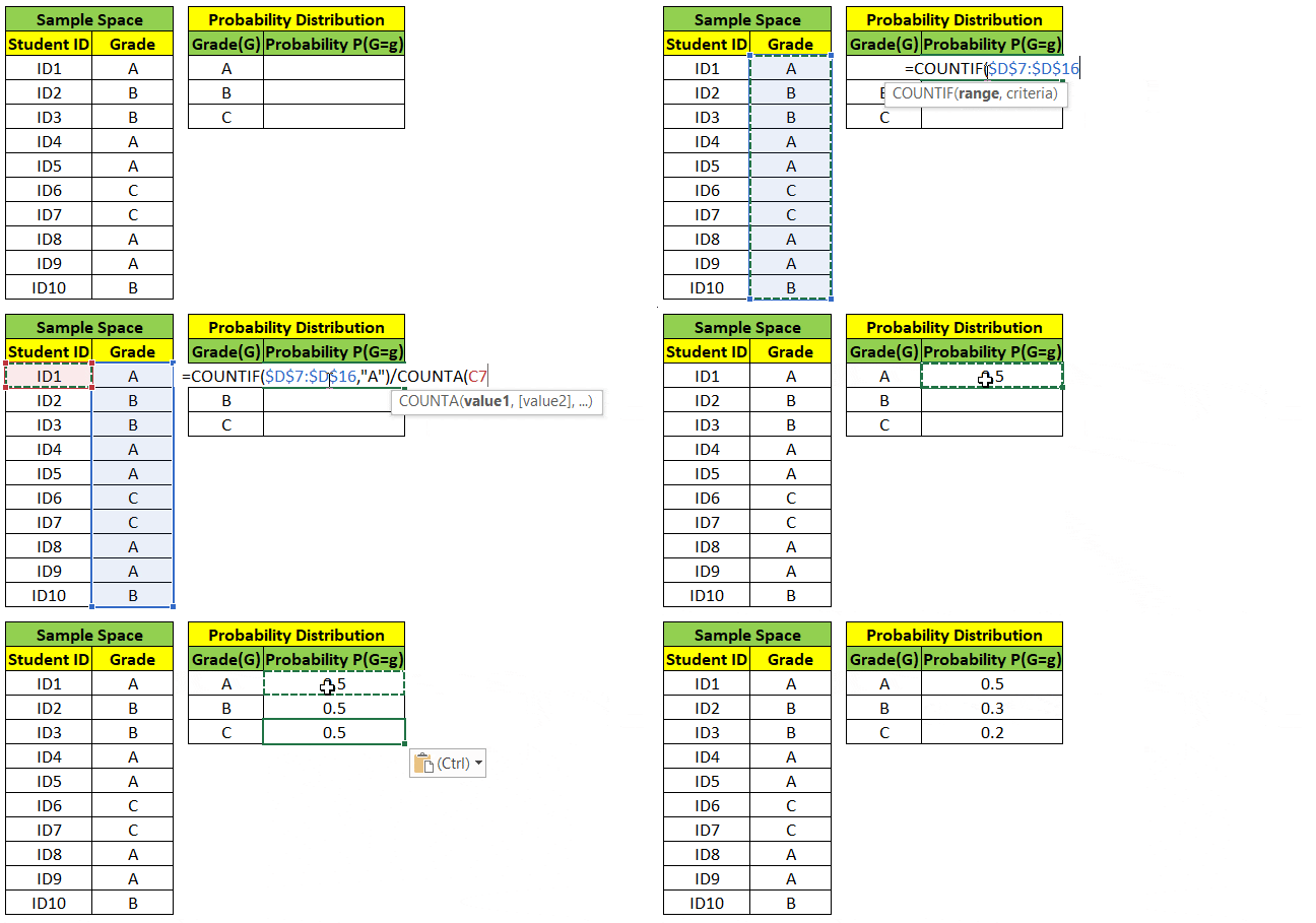
Random Variable can either take Continuous values (ex weight, height) or Discrete values (ex grade, yes/no). We can find probability distribution of Random Variable as shown below.
Introduction
Why do we recapped Random Variable ?
Given a classification problem to predict whether given image contains Text (Class 0) or contains No-Text (Class 1).
ML classification model will predict the target which is Random Variable X (taking either Class 0 or 1) with probability associated of these 2 classes. Ex: ŷ = [Class 0 : 0.4, Class 1: 0.6].
We also know the True Distribution y = [Class 0: 0, Class 1: 1] i.e. we are 100% sure that given image has Text in it.
How can we compare the predicted vs actual distribution? How sure is our predicted distribution is ? Remember we might have “n” such predictions and each time we have True Vs Predicted probability distribution.
We cannot do a simple RMSE(Root Mean Square Error) as we deal with probability values and simple RMSE will violate “Axioms of Probability”. Hence we need a different kind of loss function – enter “CROSS ENTROPY”
Expectation Value
Expected Value or Mean of a Random Variable is E(X)=μ=∑ x * P(x) i.e. random variable x multiplied by its probability. Take a look on below image for example.
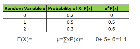
substituting values in formula, Expected Gain E(X)=μ=∑x * P(x)=0+.5+.6=1.1E(X)=μ=∑x * P(x)=0+.5+.6=1.1
Information Content
It is a basic quantity derived from the probability of a particular event occurring from a random variable.
According to Claude Shannon’s definition,
- An event with probability 100% is perfectly unsurprising and yields no information.
- The less probable an event is, the more surprising it is and the more information it yields i.e. inversely proportional IC(x) = log2(1/P(x)) = [log2 1 – log2(P(x))] = -log2(P(x)), since log1 =0
- If two independent events are measured separately, the total amount of information is the sum of the self-information’s of the individual events.
Entropy
We spoke about Random Variable which can taken different values and each values has probability thus forming distribution. Next, we looked at the information content of the event which is inversely proportional to log of probability of that event.

So to find expected information content is given as E[gain]=∑P(x=i)*(-log2(P(x))) which tells average information contained in our data called as Entropy H(x).
Subscribe to our newsletters !!
Cross Entropy
Now we are ready to discuss the topic that we are interested in – to compare 2 different distributions.
Given, a Random Variable x taking 4 different values,
x ~ [A, B, C, D]
Assume, it’s true probability associated with it represented as yi ~ P(x=A/B/C/D),
x ~ [y1, y2, y3, y4]
Hence, we can find it’s Information Content,
IC(x) ~ [-log2y1, -log2y2, -log2y3, -log2y4]
Original Entropy which gives average information content of True Distribution,
H(y) = -∑ yi * log yi where i = 1,2,3,4
Our Machine Learning model will estimate probability ŷ,
x̄ ~ [ŷ1, ŷ2, ŷ3, ŷ4]
and its information content as,
IC(x̄) ~ [-log2ŷ1, -log2ŷ2, -log2ŷ3, -log2ŷ4]
Entropy of Estimated distribution i.e. Cross Entropy,
H(y, ŷ) = -∑ yi * logŷi where i = 1,2,3,4
Our goal is to find the difference of Entropy & Cross Entropy, lead us to “KL Divergence” formula.
KL Divergence
Also known as Kullback-Leibler Divergence (KL divergence), or relative entropy – gives a score that measures the divergence of one probability distribution from another.
KL Divergence = (y||ŷ) = H(y, ŷ) – H(y)
= -∑ yi * logŷi – (-∑ yi * log yi)
= -∑ yi * logŷi + ∑ yi * log yi
in terms of ML, we need to minimize this loss for better prediction
KL Divergence = (y||ŷ) = min{-∑ yi * logŷi + ∑ yi * log yi}
Consider, we use logistic regression as our classification model (can be any algorithm), which uses Sigmoid function for prediction.
σ(x) = 1/(1+exp(-x))
= 1 / (1 + exp(-(w*x +b)) where w & b represents slope & intercept of sigmoid function
So, our KL Divergence minimization optimization is with respect to parameters w, b
KL Divergence = (y||ŷ) = min w, b {-∑ yi * logŷi + ∑ yi * log yi}
we know only ŷ which is predicted probability using sigmoid function is dependent on parameters w, b
KL Divergence = (y||ŷ) = min w, b {f(w,b) + C} i.e. True probability distribution is constant
= min w, b {-∑ yi * logŷ} = H(y, ŷ)
So, in practice entire “KL divergence equation boils down only to minimization Cross Entropy formula“.
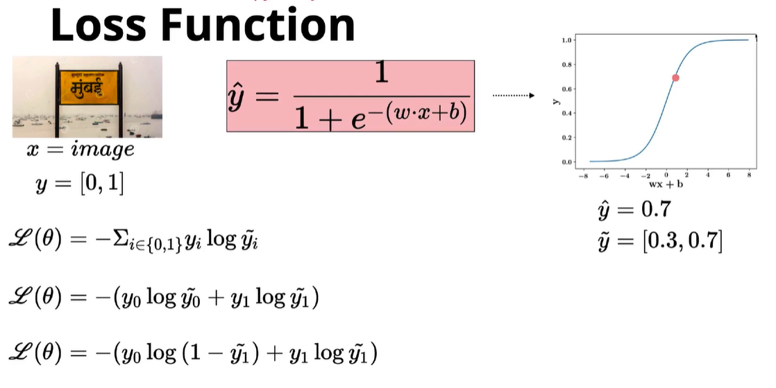
Example
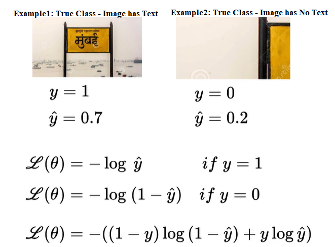
Taking our example of predicting whether image has Text or No Text.
Given, image with Text. So True Probability is [1, 0]
Say, our ML model predicted probability as [0.7, 0.3]
Substituting in Cross Entropy Formula
H(y, ŷ) = -∑ yi * logŷi
= – (1*log2(0.7) + 0*(log2(0.3))
= – (1*log2(0.7)) , since second term is 0
= -log2(0.7)
~ -logŷc, where c represents True class
So, we can “directly take negative log of predicted probability for True Class” (in our case image has Text is True Class) to find loss value.
Simplified Cross Entropy
In any case, True class can be varied. A given image may have Text or No Text & it’s true class will be varied accordingly. Hence we need to modify the formula to adjust accordingly
Conclusion
We started with why RMSE cant be used as a loss function to compare 2 different probability distributions. Hence we need for different loss functions using information theory developed by Claude Shannon.
We saw about,
Expected Value E(x) = ∑x * P(x), since x is a random variable that takes different values with probability associated with it.
Information Content IC(x) = -log2(P(x)), rare an event – more the information content
Entropy H(x) = ∑P(x=i)*(-log2(P(x))), that computes average information content using Expected value formula
KL Divergence (y||ŷ)= min w, b {-∑ yi * logŷ}, measures how one probability distribution is different than other
And approximated KL Divergence equation to Cross Entropy H(y, ŷ) = -∑ yi * logŷi , average information content of predicted probability distribution
Finally, Simplified to -((1-y)log(1-ŷ) + ylogŷ), which will work whatever may be our True distribution is….
Cross Entropy loss is almost used in all Deep Learning and Machine Learning classification models when the output is in probability for different classes. Hope you like this article, if so please share with your friends and leave a comment. Till we come back with another interesting topic, keep reading !!
- https://ainxt.co.in/deep-learning-on-types-of-activation-functions/
- https://ainxt.co.in/step-by-step-interview-guide-on-linear-regression-algorithm/
- https://ainxt.co.in/step-by-step-interview-guide-on-logistic-regression-algorithm/
- https://ainxt.co.in/guide-to-understand-basic-matrix-principles-in-depth/






[…] https://ainxt.co.in/hidden-facts-of-cross-entropy-loss-in-machine-learning-world/ […]